Anaconda 多环境

# 查看所有环境
conda info -e
# 查看当前环境详细信息
conda info

# 创建新环境
conda create -n env_name 
# 创建并指定 python 版本
conda create -n book_env python=3.6.5 --channel conda-forge


# 激活某环境
conda activate env_name
# 退出某环境
conda deactivate

# 删除环境
conda remove -n env_name --all

# 为指定环境安装包
conda install -n env_name pandas
# 查看环境所安装的包
conda list -n env_name

# 删除安装包
conda remove -n env_name numpy

准备环境及依赖

# 要安装最新的 gcc 先
brew install gcc
conda create -n book_env python=3.6.5 --channel conda-forge
conda activate book_env
#conda install -c conda-forge imbalanced-learn
conda install pip

# 超时 -default-timeout=1000
pip install -r requirements.txt

# 然后启动
jupyter lab

数据分析基础及统计学基础

数据分析

数据收集
- HTML, 爬虫
- API
- DB
- 可供下载网络资源
- 日志文件等
数据整理. 可能遇到的问题
- 人为错误的数据
- 计算错误的数据
- 异常值
- 不完整的数据
- 数据格式问题
探索性数据分析, EDA (Exploratory data analysis)
得出结论

统计学基础

概念

Sample : 样本
- 必须是随机样本. random sample . 即是没偏见的.
- 取样方法
- simple random sample : 简单随机抽样
- stratified random sample : 分层随机抽样(数据有分组)
- bootstrap sample : 从样本中随机重抽样替换后的样本. 例如, 有个 sample 为 1, 2, 4, 4, 10, 则 bootstrap sample 可能为 2, 1, 10, 4, 2 或 4, 10, 10, 2, 4 或 4, 1, 1, 4, 10 等.
Population : 总体
统计类型
- descriptive statistics : 描述性统计
- inferential statistics : 推论性统计

descriptive statistics, 描述性统计

下面描述的都是单变量的

central tendency : 集中趋势
- mean : 总体的平均值写为 $\mu$ , 样本的平均值写为 $\bar{x}$ . 公式 $\bar{x} = \frac{\sum{1}^{n} x{i}}{n}$
- 它对 outlier 值敏感
- median : 表示数据的 $50^{th}$ 百分位. 即中位数.
- 这表示 50% 的数据大于该值, 50% 的数据小于该值
- 计算公式: 从一个排序的数据中, 取中间那个
- mode : 众数
- unimodal : 单峰
- bimodal : 双峰
- multimodal : 多峰
Measures of spread : 离散度
- range : $range = max(X) - min(X)$
- variance : 方差. 总体的方差写为 $\sigma^2$ , 样本的方差写为 $s^2$
- 方差是各个数据与其算术平均数的离差平方和的平均数
- 如果想用样本方差来估算总体方差, 则除以 n-1 而不是 n , 这叫 Bessel's correction
- $s^2 = \frac{\sum_{1}^{n} (x_i - \bar{x})^2}{n-1}$
- standard deviation : 标准差.
- 由于方差的单位, 与数据的单位不一致, 所以这里转换为一至才可比较.
- $s = \sqrt{\frac{\sum_{1}^{n} (x_i - \bar{x})^2}{n-1}} = \sqrt{s^2}$
- 越小, 分布曲线越瘦; 越大, 分布曲线越肥
- Coefficient of variation, CV, 变异系数
- 标准差与平均值之比. $CV = \frac{s}{\bar{x}}$
- 它告诉我们, 标准差相对于平均值有多大
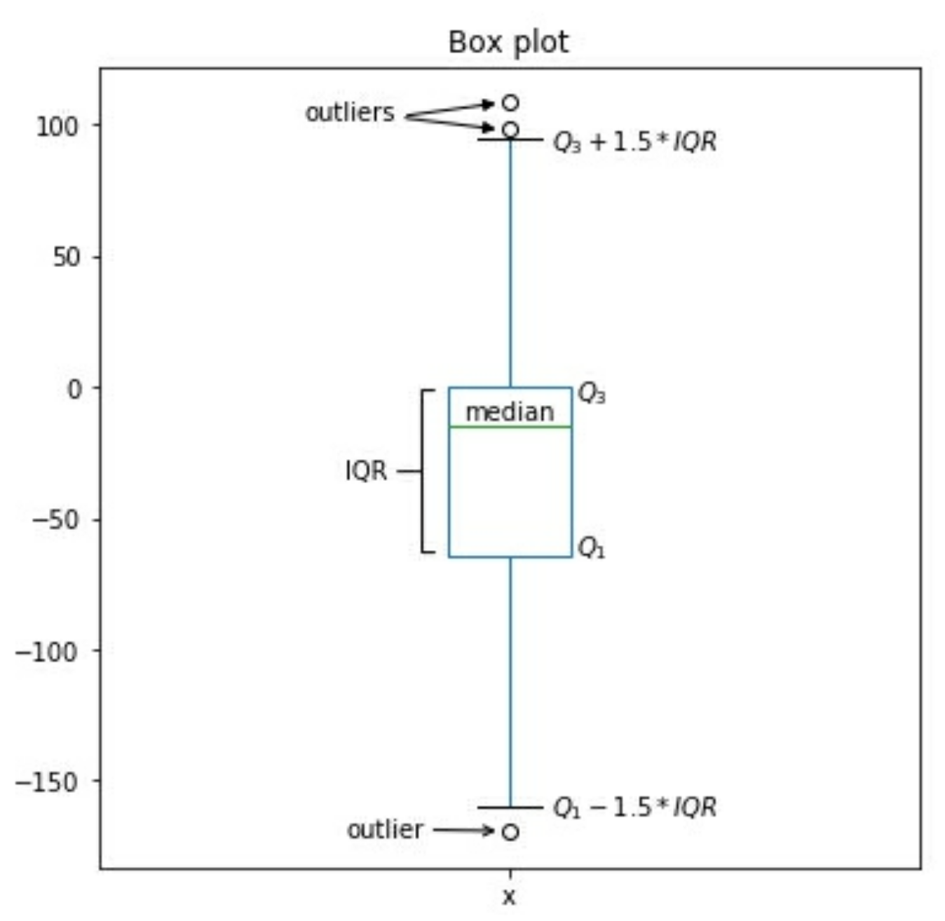
- 用于比较不同数据集的离散程度
- Interquartile range : IQR, 四分位范围
- $50^{th}$ 百分位, 也叫 $2^{nd}$ 四分位数. $Q_2$
- 百分位与四分位都叫分位数(quantiles). 百分位给出的是 100 分. 而四分位给出的四个25%(), 50%, 75%, 100%
- $Q_1 表示 25\%$, $Q_2 表示 50\%$, $Q_3 表示 75\%$, $Q_4 表示 100\%$
- $IQR = Q_3 - Q_1$
- Quartile coefficient of dispersion : QCD 四分位离散系数.
- $QCD = \frac{\frac{Q_3 - Q1}{2}}{\frac{Q_1 + Q3}{2}} = \frac{Q_3 - Q_1}{Q_3 + Q_1}$
- 用于比较不同数据集
- Summarizing data : 数据摘要. 5-number summary
quartile statistic percentile

1 $Q_0$ minimum $0^{th}$

2 $Q_{1}$ N/A $25^{th}$

3 $Q_{2}$ Median $50^{th}$

4 $Q_{3}$ N/A $75^{th}$

5 $Q_{4}$ maximum $100^{th}$
- box plot : 箱图. 它是 5-number summary 的可视化.
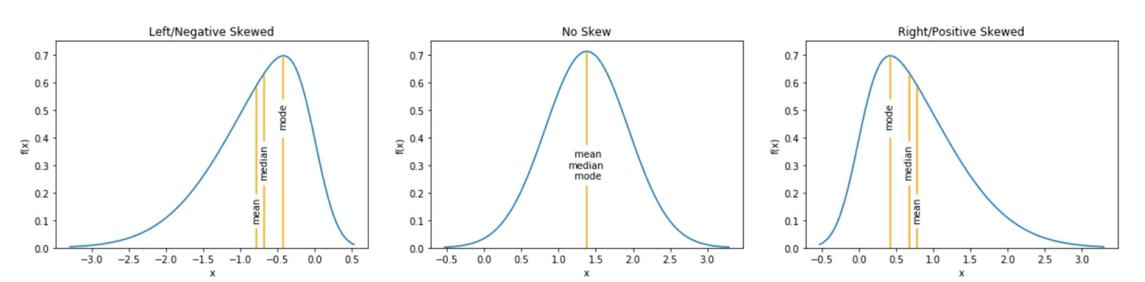
- histograms : 直方图, 通常用于离散变量 discrete variables
- kernel density estimates : KDEs , 内核密度估计. 用于连续变量. continuous variables . 它类似于直方图, 但它不用 bins , 而不画一条平滑曲线, 它表示对于连续型变量分布的概率密度函数(probability density function, PDF)的估计. PDF 值越高, 表示越可能是它. 当存在负偏态(向左倾斜)时, 表示均值 mean 小于中值 median ; 当存在正偏态(向右作料)时表示 mean 值大于中值 median ; 当没有倾斜时, 两者相等.
当我们对获得一个 <=x 的可能性时, 可以用 cumulative distribution function, CDF (累积分布函数), 它是曲线下面区域的积分.

$ CDF = F(x) = \int{-\infty}^{x} f(t)dt$ , $f(t)$ 是 PDF(概率密度函数), 并且 $\int{-\infty}^{\infty}f(t) dt = 1$

对于连续型变量, 准确得到 x 的概率为 0. 这是因为概率为 x 到 x 的积分, 结果为 0 (在曲线区域下面, 并且 0 宽度的意思).

即 $P(X = x) = \int_{x}^{x}f(t)dt = 0$

为了可视化它, 我们可以从样本中找到 CDF 的估计, 称为empirical cumulative distribution function, ECDF , 先验累积分布函数. 例如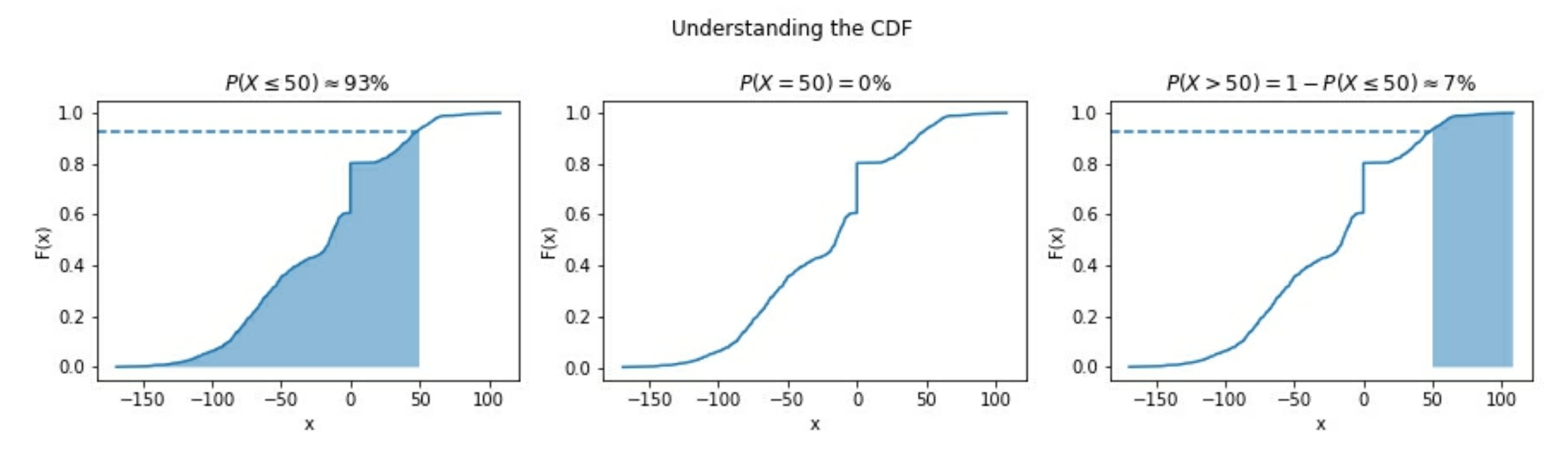
- 对于离散型分布, 我们使用 probability mass function, PMF (概率质量函数), 来代替 probability density function, PDF (概率密度函数)

	quartile	statistic	percentile
1	$Q_0$	minimum	$0^{th}$
2	$Q_{1}$	N/A	$25^{th}$
3	$Q_{2}$	Median	$50^{th}$
4	$Q_{3}$	N/A	$75^{th}$
5	$Q_{4}$	maximum	$100^{th}$

Inferential statistics , 推论性统计

我们无法控制自变量, 意味着我们无法得出因果关系

通过实验，我们可以直接影响自变量并将主题随机分配给对照组和测试组，例如A / B测试. 理想的设置应该是 double-blind (双盲)

用来估计总体参数的统计量称为估计量 estimator , 它是一个随机变量. 比如, 用样本平均数 $\bar x$ 去估计总体平均数 $\mu$ , 这里的 $\bar x$ 是 $\mu$ 的估计量. 如果用估计量的单一值作为总体参数的估计值, 那就是点估计 point estimation . 如果指定估计量的一个取值范围都作为总体参数的估计, 那便称区间估计 interval estimation .

confidence coefficient : 置信系数: 所构建的敬意可以包含总体参数的概率. 这个概率越高, 估计的可靠程度越高, 做出决策的把握也就越大. $置信系数 = 1 - \alpha $ , 其中, $\alpha$ 是显著性水平.

condidence intervals : 置信区间. 按照一定置信系数所求得的估计区间. 该区间提供点估计和周围的误差范围. 通常以 95% 作为置信水平. 它是随机变量.

常见的分布

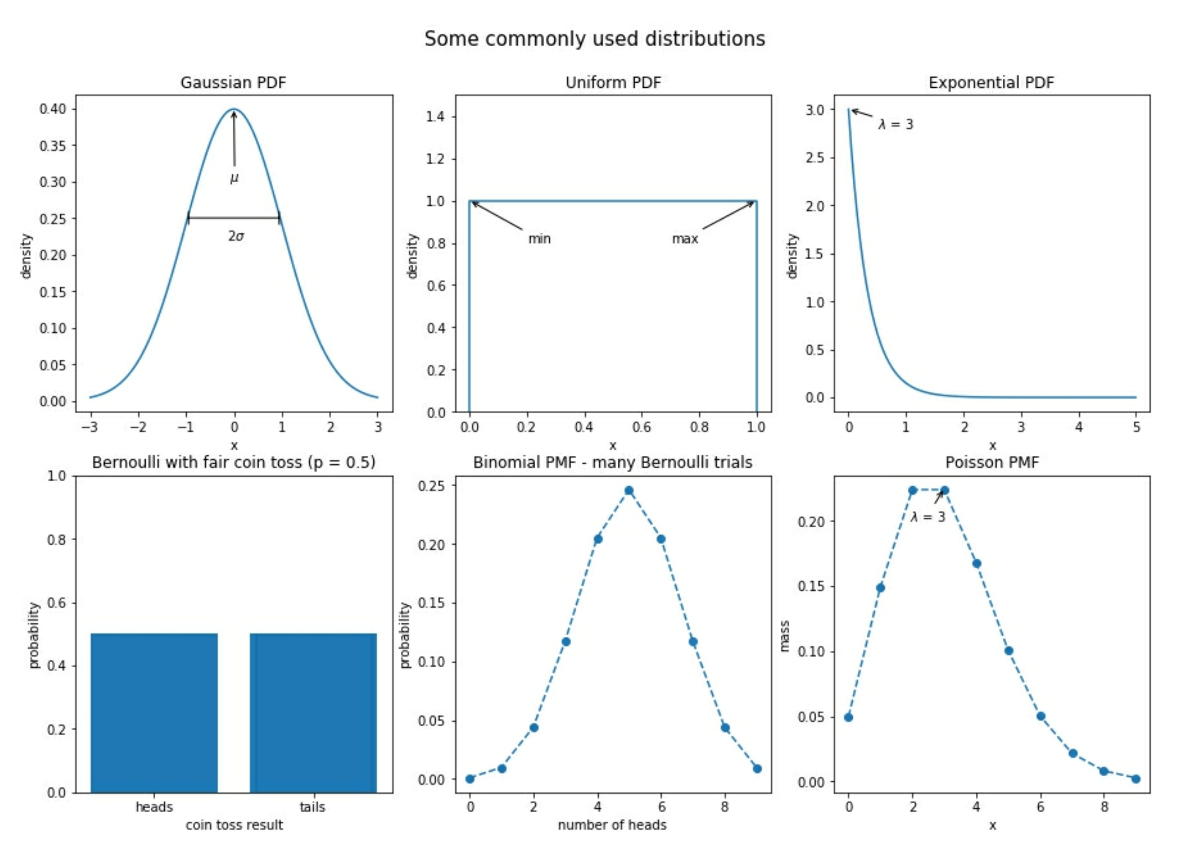
有一些常见的概率分布

Gaussian 高斯分布

或叫正太分布(normal). 看上去像一个钟形曲线. 它的参数由

mean ( $\mu$ )平均值
standard deviation ($\sigma$) 标准差来决定.

标准的正态分布standard normal(Z) 是由 mean 平均值为 0, 以及 standard deviation 标准差为 1组成的. 许多自然界中的东西都呈正态分布.

Poisson 泊松分布

它是一种离散分布. 通常用于对到达进行建模.

在到达之间的时间, 可以被指数分布(exponential distribution)进行建模.

二者都可以通过它们的 mean , 以及 lambda ($\lambda$) 来定义.

uniform 均匀分布

在它的范围内, 每个值的概率是相等的. 当我们使用一个随机数来模拟单个成功或失败结果时, 这叫 Bernoulli trial (伯努利试验). 它的参数是成功的概率 $p$ . 当我们多次 n 运行相同的实验时, 成功的总数就是一个二项式(binomial)随机变量.

Bernoulli 和 Binomial 都是离散分布

常见分布的可视化

数据缩放 scaling data

min-max scaling

$x_{scaled} = \frac{x - min(X)}{range(X)}$

standardize data

标准化数据

$z_i = \frac{x_i - \bar x}{s}$

即元素与平均值之差, 再除以标准差. 结果就是著名的 Z-score .

我们得到的均值为 0 且标准差(和方差)为 1 的归一化分布. Z-score 告诉我们每个观察值与均值有多少标准差; 平均值的 Z-score 为 0. 而低于平均值的 0.5 标准差的观察值的 Z-score 为 -0.5

量化变量之间的关系

covariance 协方差, COV

$$ cov(X, Y) = E[ (X - E[X]) (Y - E[Y]) ] $$

E[X] 表示 X 的期望

Pearson correlation coefficient

Pearson 相关系数, 符号为 $\rho$ $$ \rho _{X, Y} = \frac{cov(X, Y)}{s_X s_Y} $$ 这会标准化 COV (协方差) 并且结果为统计范围的 -1 ~ 1

1 表示完全正相关
-1 表示完全负相关
0 附近表示没有相关
绝对值在 1 附近表示强相关
绝对值 小于 0.5 表示弱相关

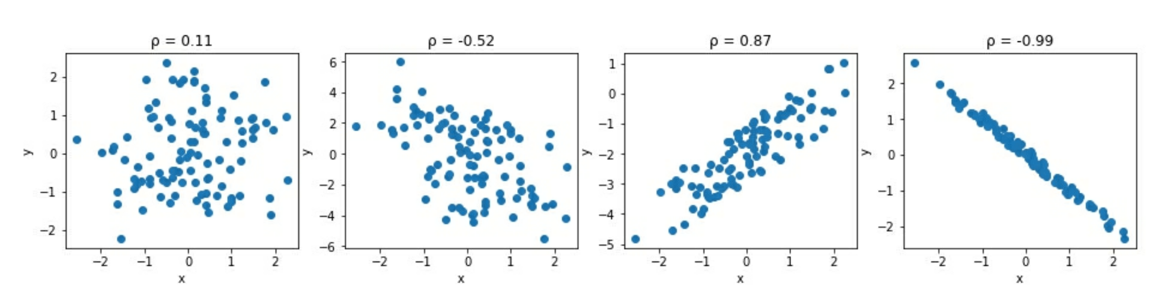
注意, 相关性并不等同于因果性

ARIMA

对于时序数据, 我们常见的建模方法有指数平滑 exponential smoothing , 以及 ARIMA 家族模型

autoregressive, AR . 自回归.
- 利用了以下事实: 时间 t 的观察与之前的观察相关
- 注意, 不是所有的时序都是 AR 的
integrated, I. 整合. 它关注差异(differenced data)数据 , 或者数据从一个时间到另一个时间的变化. 比如如果我们关注一个 lag , 则差异数据的值为 t - 1
moving average, MA . 移动平均. 它使用 sliding window (滑动窗口) 来计算最近 x 个观察值的平均值, x 是 sliding window 的长度

exponential smoothing, 指数平滑

它允许我们将更多的权重放在最近的数据, 更少的权重放在旧的数据. (相对于我们的预测位置)

各种常见统计函数

import random
import numpy as np
import pandas as pd
random.seed(0)
salaries = [round(random.random()*1000000, -3) for _ in range(100)]

data = pd.Series(salaries)

# 概要
data.describe()

# mean 平均数
data.mean()

# median 中位数
data.median()

# mode 众数
data.mode()

# var 方差
data.var()

# std 标准差
data.std()

# range
[data.min(), data.max(), data.max() - data.min()]

# coefficient of variation, CV
data.std() / data.mean()

# interquartile range. IQR
Q1 = data.quantile(0.25)
Q3 = data.quantile(0.75)
IQR = Q3 - Q1
print(Q3, Q1, IQR)

# quartile coefficent of dispersion, QCD
(Q3 - Q1) / (Q3 + Q1)

# min-max scaling data
(data - data.min()) / (data.max() - data.min())

# standardizing data. 元素与平均值之差, 再除以标准差
(data - data.mean()) / data.std()

# covariance, COV
data.cov(data)

# Pearson correlation coefficient. 相关性. 默认为 pearson
data.corr(data)
data.corr(data, method='pearson')
data.corr(data, method='spearman')
data.corr(data, method='kendall')

Pandas Data Structures

主要有 Series 和 DataFrame . 它们都包含另一个 data struct : Index .

注意, Pandas 的 data struct 是构建于 Numpy 之上的.

上面提到的 data struct , 都是通过 Python 的 classes 来创建的, 当创建一个时, 它们称为 objects 或 instances . 所以, 它们有时会使用 object 自身的 method ; 有时会将它们作为参数传递给其他 function

所以, Pandas 实质是一个 object 或 instance. 它们有

method
attribute

NumPy 风格

简单还好, 复杂一点就比较笨重了

import numpy as np

data = np.genfromtxt(
    'data/example_data.csv', delimiter=';', 
    names=True, dtype=None, encoding='UTF'
)

data

# 获取第三列的最大数
max([row[3] for row in data])

# 将它变成 dict
array_dict = {}
for i, col in enumerate(data.dtype.names):
    array_dict[col] = np.array([row[i] for row in data])
array_dict

# 获取字典最大值的所有信息
np.array([value[array_dict['mag'].argmax()] for key, value in array_dict.items()])

Series

单一类型的数组( NumPy 的也是). 你可以想像为电子表格的一列

它有一个列名

以及相同的数据类型

import pandas as pd

place = pd.Series(array_dict['place'], name='place')
place

这时, 默认它还含有 Index 对象, 对应相应的行号(从 0 开始, 偏移为 1). Series 常见的属性有

name : Series 对象的名字
dtype : Series 对象的数据类型
shape : Series 对象里一行数据里的维度(行数)
index : Series 对象的 Index Object
values : Series 对象的数据作为 NumPy 数组

https://pandas.pydata.org/pandas-docs/stable/reference/api/pandas.Series.html

Index

Index class 是 row label (行标签), 可以通过行来选择. 取决于 Index 的类型, 可以是

Row Number : RangeIndex(start=0, stop=5, step=1) . 这也是默认的类型.
Date
String

可以通过 Series.index 来获取 index 对象.

Index 也是建在 NumPy 的 array 之上. 可以通过 Series.index.values 属性来获取 NumPy Array .

Index 常见的属性有

name
dtype
shape
values
is_unique

Pandas 中, 两个 Series 之间的算术运算是在 Index 是否匹配之上的. 例如

pd.Series(np.linspace(0, 10, 5)) + pd.Series(np.linspace(0, 10, 5), index=pd.Index([1,2,3,4,5]))

即

0     0.0                1     0.0              0     NaN    
1     2.5                2     2.5              1     2.5 
2     5.0          +     3     5.0       =      2     7.5              
3     7.5                4     7.5              3    12.5
4    10.0                5    10.0              4    17.5
dtype: float64           dtype: float64         5     NaN     
                                                dtype: float64

而 NumPy 是基于元素的位置来进行运算的

DataFrame

它是建于 Series 之上的. 可以想像它是一个电子表格, 有许多列(相对地, Series 是一列), 每一列都有相同的数据类型.

DataFrame 常见的属性有

dtypes
shape
index : DataFrame 的 Index 对象
columns : DataFrame 的列名(作为一个 Index 类型对象)
values : DataFrame 中的所有值作为 NumPy 数组

DataFrame 之间的操作, 是基于 Index 匹配以及 Column 匹配( Series 则只在 Index 匹配) 之上的.

填充数据到 DataFrame

Series 是 DataFrame 的必要要素, 它是 DataFrame 的某一列

Python Object -> DataFrame

# Series -> DataFrame
pd.Series(np.linspace(0, 10, num=5), name='hello').to_frame()

# 多行多列
pd.DataFrame(
    {
        'random': np.random.rand(5),
        'text': ['hot', 'warm', 'cool', 'cold', None],
        'truth': [np.random.choice([True, False]) for _ in range(5)]
    }, 
    index=pd.date_range(
        end=datetime.date(2019, 4, 21),
        freq='1D',
        periods=5, 
        name='date'
    )
)

# list dict  -> DataFrame
pd.DataFrame([
    {'mag' : 5.2, 'place' : 'California'},
    {'mag' : 1.2, 'place' : 'Alaska'},
    {'mag' : 0.2, 'place' : 'California'},
])

# list tuple -> DataFrame
list_of_tuples = [(n, n**2, n**3) for n in range(5)]
pd.DataFrame(
    list_of_tuples, 
    columns=['n', 'n_squared', 'n_cubed']
)

# numpy array -> DataFrame
pd.DataFrame(
    np.array([
        [0, 0, 0],
        [1, 1, 1],
        [2, 4, 8],
        [3, 9, 27],
        [4, 16, 64]
    ]), columns=['n', 'n_squared', 'n_cubed']
)

File -> DataFrame

CSV 文件: df = pd.read_csv('data/earthquakes.csv')
Excel 文件: pd.read_excel()
JSON 文件: pd.read_json()
TSV 文件: pd.read_csv(sep='\t')

常见的参数

sep : 分割符
header : 列名所在的行号. 默认是 infer , 即让 Pandas 自动判断
names : 显式指定列名
index_col : 作为 index 的列
usecols : 只读取哪些列
dtype : 为列指定类型
converters : 指定列的数据转换函数
skiprows : 跳过多少行
nrows : 一次读取多少行
parse_dates : 自动将包含日期的列转成 datetime object
chunksize : 分块读取文件
compression : 直接读取压缩的文件而不用解压
encoding : 指定文件编码

将 DataFrame 保存到文件:

# 注意, index 的数据默认也是写入的
df.to_csv('outpupt.csv', index=False)

Database -> DataFrame

# 写入DB. to_sql(), if_exists='replace' 表示, 如果存在则替换
import sqlite3

with sqlite3.connect('data/quakes.db') as connection:
    pd.read_csv('data/tsunamis.csv').to_sql(
        'tsunamis', connection, index=False, if_exists='replace'
    )
    
# 从 DB 读取
with sqlite3.connect('data/quakes.db') as connection:
    tsunamis = pd.read_sql('SELECT * FROM tsunamis', connection)

API -> DataFrame

import datetime
import pandas as pd
import requests

yesterday = datetime.date.today() - datetime.timedelta(days=1)
api = 'https://earthquake.usgs.gov/fdsnws/event/1/query'
payload = {
    'format' : 'geojson',
    'starttime' : yesterday - datetime.timedelta(days=26),
    'endtime' : yesterday
}
response = requests.get(api, params=payload)

# let's make sure the request was OK
print(response.status_code)

earthquake_properties_data = [data['properties'] for data in earthquake_json['features']]
df = pd.DataFrame(earthquake_properties_data)

Inspecting a DataFrame Object

DataFrame 的每一列都是一个 Series

# 是否为空(即没数据)
df.empty

# 形状 (nrows, ncols)
df.shape

# 查看前N 行数据. N不写则为 5
df.head(N)

# 查看后 N 行数据. N不写则为5
df.tail(N)

# 查看所有列
df.columns

# 查看数据类型
df.dtypes

# 详细信息
df.info()

# 概要统计信息
df.describe()

# 如果是 object 类型, 则统计信息不像数字统计那样了
# count, unique(表示去重后的个数), top (众数), freq(众数出现的频率)
df.describe(include=np.object)
df.describe(include='all')

# 只看某列概要
df['colName'].describe()

以下方法对于 Series 和 DataFrame 都适用:

method	des	Data type
`count()`	非 null 出现的次数	Any
`nunique()`	唯一值的数量	Any
`sum()`		number or boolean
`mean()`		number or boolean
`median()`		number
`min()`		number
`idxmin()`	Index 中的最小值	Number
`max()`		number
`idxmax()`	Index 中的最大值	number
`abs()`		number
`std()`		number
`var()`		number
`cov()`		number
`corr()`		number
`quantile()`	获取指定分位数	Number
`cumsum()`	累积和	number or boolean
`cummin()`	累积最小值	number
`cummax()`	累积最大值	Number

Series 有的方法

method	des
`unique()`	获取唯一值
`value_counters()`	获取频率计数表
`mode()`	获取众数

Index 有的方法

method	des
`argmax()/argmin()`	查找 index 的最大/最小值位置
`contains()`
`equals()`	跟另一个 Index 对象比较是否相等
`isin()`	给定一些索引值的 list, 并返回 boolean 的数组, 判断index 是否在指定值中
`max()/min()`	查找 Index 的最大/最小值
`nunique()`	唯一值的个数
`to_series()`	从 Index 中生成一个 Series 对象
`unique()`	查找唯一值
`value_counts()`	生成一个唯一值的频率表

提取数据子集

Selection

获取列. column selection

# 获取一列
df['msg']

# 多列
df[['msg', 'title']]

# 获取符合条件的列. 获取 title, time 列, 以及所有列名以 mag 开头的列
df[
    ['title', 'time']
    + [col for col in df.columns if col.startswith('mag')]
]

Slicing

获取行. row slicing

# 注意, 行号是从 0 开始. 这里即获取 第 100 到 102 行的数据, 共 3 行
df[100:103]

# 组合列行
df[['time', 'title']][100:103]

Indexing

loc[] : 使用 label-based
iloc[] : 使用 integer-based

所有的 indexing method, 第一个参数是 row indexer, 然后到 column indexer . 例如

# 所有行或列, 则写成 :
df.loc[row_indexer, column_indexer]

df.loc[:, 'title']
df.loc[10:15, ['title', 'mag']]

# 通过 integer 来索引, 列也是从 0 开始
df.iloc[10:15, [19, 8]]

df.iloc[10:15, 8:10]

查找 scalar value (标量值) , 可以用 at[] 以及 iat[]

# 获取第 10 行, 列为 mag 的值
df.at[10, 'mag']

# 获取第 10 行, 第 8 列的值. (都是从 0 开始)
df.iat[10, 8]

Filtering

Boolean masks : 返回与数据相同结构的 shape, 但里面是用 True/False 填充的. 例如

df['mag'] > 2

# 通过它可以进行条件选择 df. 
df[df['mag'] > 2]

# loc 也可以处理 boolean masks
df.loc[df['mag'] > 2, ['mag', 'title']]

# 多条件, 要注意括号. &, |
df.loc[(df['mag'] > 2) & (df['alert'] == 'red'), ['mag', 'title']]

# 如果是字符串
df.loc[
    (df.place.str.contains('Alaska')) & (df.alert.notnull()),
    ['alert', 'mag', 'magType', 'title', 'tsunami', 'type']
]

# 数值范围
df.loc[
    df.mag.between(6.5, 7.5),
    ['alert', 'mag', 'magType', 'title', 'tsunami', 'type']
]

# isin
df.loc[
    df.alert.isin(['orange', 'red']),
    ['alert', 'mag', 'magType', 'title', 'tsunami', 'type']
]

# 获取某列最大, 最小值的行
df.loc[
    [df.mag.idxmin(), df.mag.idxmax()],
    ['alert', 'mag', 'magType', 'title', 'tsunami', 'type']
]

添加或删除数据

添加

# 添加新列
df['ones'] = 1
df['mag_negative'] = df.mag < 0


# 按行拼接
pd.concat([tsunami, no_tsunami])
tsunami.append(no_tsunami)

# 按列拼接
additional_columns = pd.read_csv(
    'data/earthquakes.csv', usecols=['tz', 'felt', 'ids', 'time'], index_col='time'
)
pd.concat(
    [df.head(2), additional_columns.head(2)], axis=1
)

# 指定连接方式, join 参数
pd.concat(
    [tsunami.head(2), no_tsunami.head(2).assign(type='earthquake')], join='inner'
)

删除

del df['ones']

# 弹出并移除某列
one = df.pop('ones')

# 直接删除多行或多列. 
# 删除前 2 行. 默认是按行删除的. axis=0
df.drop([0, 1])

# 删除多列
df.drop(columns=['title', 'mag'])

默认情况下, drop 会返回一个新的 dataframe, 如果相在原 dataframe 直接修改, 可传一个参数 inplace=True

使用 Pandas 进行数据分析

Data Wrangling

它是将输入的数据进行格式化处理, 使我们可以有意义地分析它. 也称为Data manipulation 通常有三个任务(没有固定顺序的, 看情况)

Data cleaning
- Renaming
- Sorting and reordering
- Data type conversions
- Deduplicating data
- Addressing missing or invalid data
- Filtering to the desired subset of data
Data transformation

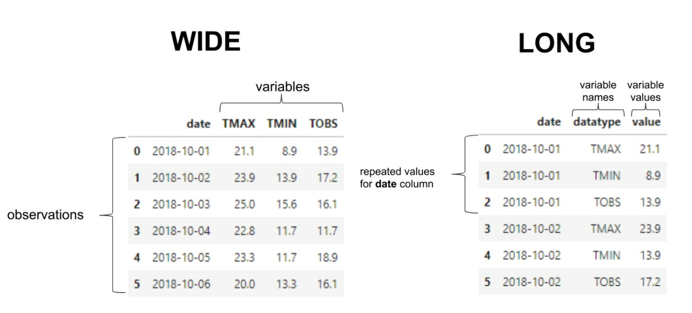
数据分 wide format (这个对数据分析和 DB 设计更好)和 long format (灵活性更好). Pandas 期望它的数据是 wide format 以便进行可视化.

Data enrichment
- Adding new columns
- Binning
- Aggregating
- Resampling

cleaning data

renaming columns

# 查看原列名
df.columns

# 重命名列名. 大部分情况 df 返回的是新 dataframe, 所以这里传一个 inplace, 表示在原 df 上直接修改
df.rename(columns={'old_name':'new_name','old_name1':'new_name1'}, inplace=True)

# 转换为大写
df.rename(str.upper, axis='columns').columns

Type conversion

# 查看原数据类型
df.dtypes

# 转换某列, 例如日期列 date
df.loc[:, 'date'] = pd.to_datetime(df['date'])

# 在读取 CSV 时直接设置
eastern = pd.read_csv(
    'data/nyc_temperatures.csv', index_col='date', parse_dates=True
).tz_localize('EST')
eastern.head()

# 处理日期的多种方法. 转换时区:
eastern.tz_convert('UTC').head()

# 以月份为间隔 yyyy-MM
eastern.to_period('M').index

# yyyy-MM-01
eastern.to_period('M').to_timestamp().index

# 将索引转换为 datetime
df.index = pd.to_datetime(df.index)

使用 assign 方式

new_df = df.assign(
    date=pd.to_datetime(df.date),
    temp_F=(df.temp_C * 9/5) + 32
)
new_df.dtypes

使用 astype 方式

df = df.assign(
    date=pd.to_datetime(df.date),
    temp_C_whole=df.temp_C.astype('int'),
    temp_F=(df.temp_C * 9/5) + 32,
    temp_F_whole=lambda x: x.temp_F.astype('int')
)
df.head()

category 类型

df_with_categories = df.assign(
    station=df.station.astype('category'),
    datatype=df.datatype.astype('category')
)
df_with_categories.dtypes

Ordering, reindexing, sorting data

#根据某列,  desc 降序
df.sort_values(by='temp_C', ascending=False).head(10)

# 根据多列排序
df.sort_values(by=['temp_C', 'date'], ascending=False).head(10)

# 获取根据某列排序的, 前 N 行
df.nlargest(n=5, columns='temp_C')

根据 index 来排序

df.nlargest(n=5, columns='temp_C')
df.nlargest(n=5, columns='temp_C')

重新设置 index

df[df.datatype == 'TAVG'].head().reset_index()

# 直接在原 df 修改
df.set_index('date', inplace=True)

reindex : 表示在原有的 index 基础上, 以另一个 index 作为对齐基准

sp.reindex(
    bitcoin.index, method='ffill'
).head(10)


# 对齐时, 其他字段的数据填充方式
sp_reindexed = sp.reindex(
    bitcoin.index
).assign(
    volume=lambda x: x.volume.fillna(0), # put 0 when market is closed
    close=lambda x: x.close.fillna(method='ffill'), # carry this forward
    # take the closing price if these aren't available
    open=lambda x: np.where(x.open.isnull(), x.close, x.open),
    high=lambda x: np.where(x.high.isnull(), x.close, x.high),
    low=lambda x: np.where(x.low.isnull(), x.close, x.low)
)
sp_reindexed.head(10).assign(
    day_of_week=lambda x: x.index.day_name()
)

Restructing the data

Transpose DataFrames

# 行列转置
df.head().T

Pivoting DataFrames

long format -> wide format

注意, Pivot 方法期待的数据是 single index 的

pivoted_df = long_df.pivot(index='date', columns='datatype', values='temp_C')
pivoted_df.head()

# 多列. 这也称为 Hierarchical index
pivoted_df = long_df.pivot(index='date', columns='datatype', values=['temp_C', 'temp_F'])
# 获取. temp_C 分组下的 TMIN 列
pivoted_df['temp_C']['TMIN']


# 或用 pd 的函数
pd.pivot( index=long_df.date, columns=long_df.datatype, values=long_df.temp_C ).head()

MultiIndex

multi_index_df = long_df.set_idnex(['date', 'datatype'])
multi_index_df.index
multi_index_df.head()

# 如果想进行 pivot , 则要 unstack()
unstacked_df = multi_index_df.unstack()

默认情况下, unstack() 会将 index 的最内层移出到列 columns

Melting DataFrames

wide format -> long format Melting 与 Pivot 的逆操作. 可直接调用 melt() 方法转为 long format . 要指定的参数有

id_vars : 在 wide format 的数据中, 要唯一标识一行的列
value_args : 包含变量的列(即要将这些列从 wide format -> long format )
var_name : 可选参数. 变成 long format 后的列名.

value_name :可选参数. 对应的值的列名.

melted_df = wide_df.melt(
id_vars='date',
value_vars=['TMAX', 'TMIN', 'TOBS'],
value_name='temp_C',
var_name='measurement'
)
melted_df.head()

与 pivot 的 unstack() 相比, melting data 有个 stack() 方法, 注意它返回的是 Series

wide_df.set_index('date', inplace=True)
stacked_series = wide_df.stack()
stacked_series.head()

# 将 Series -> DataFrame
stacked_df = stacked_series.to_frame('values')
stacked_df.head()

Handling duplicate, missing, or invalid data

概要查看

# 先看个大概
df.head()
df.tail()
df.describe()
df.info()

处理 `null` value

pd.isnull()
pd.isna()

df.isnull()
df.isna()

# 过虑出 null 或 na
contain_nulls = df[
    df.SNOW.isnull() | df.SNWD.isna()\
    | pd.isnull(df.TOBS) | pd.isna(df.WESF)\
    | df.inclement_weather.isna()
]

contain_nulls.head(10)

# 检查某列包含 null 的行数. 必须是调用 isna , isnull , 而不能直接比较
df[df.inclement_weather.isna()].shape[0]
df[df.SNWD.isin([-np.inf, np.inf])].shape[0]

处理重复行

df.duplicated()

默认的 keep 参数是 first , 如果数据出现多于一次, 则只返回除了重复出现的第一行数据外的数据. (即只会返回有重复的数据, 然后除去重复的第一行数据, 返回其他行的数据)

如果 keep 参数是 False : 则返回所有重复的行的全部数据

df[df.duplicated()].shape[0]

# 指定的列组合是否有重复. 即 duplicated 的第一个参数
df[df.duplicated(['date', 'station'])].shape[0]

Mitigating the issues

dropna

# 删除包含 na 的行
df.dropna()

# 删除所有列都是 na 的行
df.dropna(how='all')

# 删除指定列都是 na 的行
df.dropna(how='all', subset=['SNOW','SNWD'])

fillna

ffill to forward fill

bfill to back fill

df.fillna(0, inplace=True)

# 填充方式
df_deduped.assign(
    TMAX=lambda x: x.TMAX.replace(5505, np.nan).fillna(method='ffill'),
    TMIN=lambda x: x.TMIN.replace(-40, np.nan).fillna(method='ffill')
).head()

# 以均值填充
df_deduped.assign(
    TMAX=lambda x: x.TMAX.replace(5505, np.nan).fillna(x.TMIN.median()),
    TMIN=lambda x: x.TMIN.replace(-40, np.nan).fillna(x.TMIN.median()),
    # average of TMAX and TMIN
    TOBS=lambda x: x.TOBS.fillna((x.TMAX + x.TMIN) / 2)
).head()

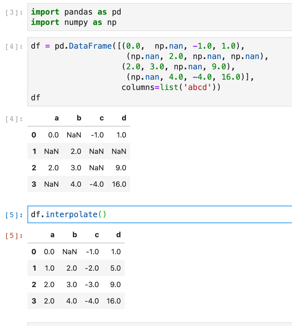
# 另一种是使用 interpolate 插值
df_deduped.assign(
    # make TMAX and TMIN NaN where appropriate
    TMAX=lambda x: x.TMAX.replace(5505, np.nan),
    TMIN=lambda x: x.TMIN.replace(-40, np.nan),
    date=lambda x: pd.to_datetime(x.date)
).set_index('date').reindex(
    pd.date_range('2018-01-01', '2018-12-31', freq='D')
).apply(
    lambda x: x.interpolate()
).tail(10)

interpolate

它的方法签名

df.interpolate(
    method='linear',
    axis=0,
    limit=None,
    inplace=False,
    limit_direction='forward',
    limit_area=None,
    downcast=None,
    **kwargs,
)

Aggregating Pandas DataFrame

Database-Style

Quering DataFrame

可以用的逻辑

or 或 and , 注意是小写的

或用符号

| 或 &

weather = pd.read_csv('data/nyc_weather_2018.csv')

# 等同于 DB 的 
# SELECT * FROM weather WHERE datatype == "SNOW" AND value > 0
snow_data = weather.query('datatype == "SNOW" and value > 0')
snow_data.head()

Merging DataFrames

Join 的四种类型

full (outer)
left
right

inner : 这是 dataframe 的默认方式

# 如果两个 dataframe 要 join 的列名不同, 则要指定
inner_join = weather.merge(station_info, left_on='station', right_on='id')

# 如果两个dataframe 列名不同, 也可先处理为相同后再 join
weather.merge(station_info.rename(dict(id='station'), axis=1), on='station').sample(5, random_state=0)

# left 和 right
left_join = station_info.merge(weather, left_on='id', right_on='station', how='left')

right_join = weather.merge(station_info, left_on='station', right_on='id', how='right')

# outer, 即 full. indicator 参数表示添加多一列, 表示该行是哪些数据组合成的
outer_join = weather.merge(
station_info[station_info.name.str.contains('NY')], 
left_on='station', right_on='id', how='outer', indicator=True
)


# 指定按索引来 join
valid_station.merge(
station_with_wesf, left_index=True, right_index=True
)

# 两个 dataframe 相同的列, 指定不同的后缀
valid_station.merge(
station_with_wesf, left_index=True, right_index=True, suffixes=('', '_?')
)

索引的集合操作

# 先在各自的 dataframe 设置为要指定集合列的索引
weather.set_index('station', inplace=True)
station_info.set_index('id', inplace=True)

# 交集
weather.index.intersection(station_info.index)

# 差集
weather.index.difference(station_info.index)

# 并集
weather.index.unique().union(station_info.index)

DataFrame operations

算术运算

fb.assign(
    abs_z_score_volume=lambda x: x.volume.sub(x.volume.mean()).div(x.volume.std()).abs()
).query('abs_z_score_volume > 3')

(fb > 215).any()

binning and thresholds

binning 或叫 discretizing (从连续到离散)

binning 的理解:

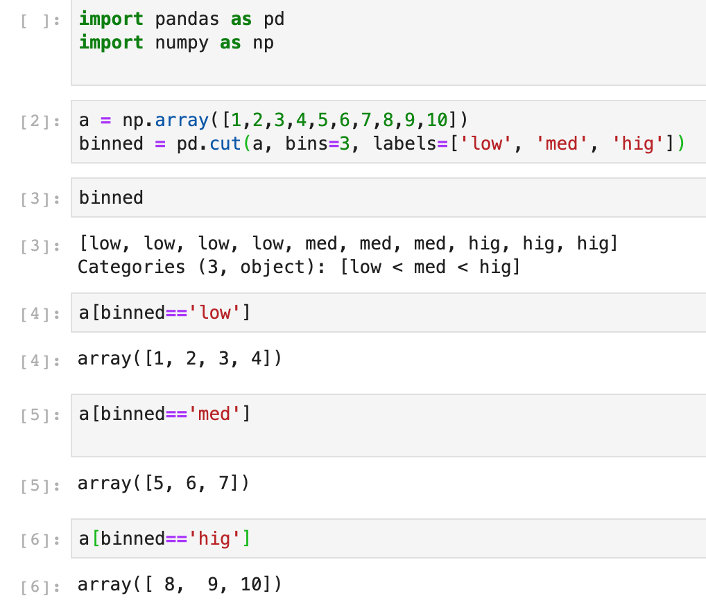
Pandas 提供了 pd.cut() 函数来基于 value 进行 binning (equal-width)

# bins=3 表示基于值的大小, 分成 3 份
volume_binned = pd.cut(fb.volume, bins=3, labels=['low', 'med', 'high'])

# 也可指定. bins=[n1, n2...n], 则 lable 有 n-1 个
red_wine['high_quality'] = pd.cut(red_wine.quality, bins=[0, 6, 10], labels=[0, 1])

# 然后获取
fb[volume_binned == 'high'].sort_values(
    'volume', ascending=False
)

# 也可以指定 bins 的序列
ml_df.assign(
    mag_bin=lambda x: pd.cut(x.mag, np.arange(0, 10))
).mag_bin.value_counts()

pd.qcut() 函数基于分位数来进行 binning (Quantile-based)

# q=4, 表示基于值的分位数, 分成 4 等份.  [0, .25, .5, .75, 1.]
volume_qbinned = pd.qcut(fb.volume, q=4, labels=['q1', 'q2', 'q3', 'q4'])

Applying function

当我们想在 dataframe 中所有的列都执行相同的代码时, 可以用 apply() 方法

oct_weather_z_scores = central_park_weather.loc[
    '2018-10', ['TMIN', 'TMAX', 'PRCP']
].apply(lambda x: x.sub(x.mean()).div(x.std()))
oct_weather_z_scores.describe().T

注意, Pandas 与 NumPy 是设计用于向量操作的. 非向量的操作, 尽可能避免

Window calculations

`rolling()`

通过 rolling, 它有一个 sliding window 来计算

central_park_weather['2018-10'].assign(
    rolling_PRCP=lambda x: x.PRCP.rolling('3D').sum()
)

central_park_weather['2018-10'].rolling('3D').mean()

对不同的列, 应用不同的聚合函数

central_park_weather['2018-10-01':'2018-10-07'].rolling('3D').agg(
    {'TMAX': 'max', 'TMIN': 'min', 'AWND': 'mean', 'PRCP': 'sum'}
)

`expanding()`

表示累积计算. 即表示以当前点数据及之前的所有数据来进行相应的函数计算

central_park_weather['2018-10-01':'2018-10-07'].expanding().agg(
    {'TMAX': np.max, 'TMIN': np.min, 'AWND': np.mean, 'PRCP': np.sum}
)

`ewm()`

指数加权移动函数.

备注: 这个还没弄懂….

fb.assign(
    close_ewma=lambda x: x.close.ewm(span=5).mean()
)

Aggregations with Pandas and NumPy

设置 Pandas 显示格式

pd.set_option('display.float_format', lambda x: '%.2f' % x)

Summarizing DataFrames

直接在 DataFrame 上执行聚合

fb.agg({
    'open': np.mean, 
    'high': np.max, 
    'low': np.min, 
    'close': np.mean, 
    'volume': np.sum
})

也可以在某列上执行多个聚合函数

fb.agg({
    'open': 'mean',
    'high': ['min', 'max'],
    'low': ['min', 'max'],
    'close': 'mean'
})

Using Groupby

fb.groupby('trading_volume').mean()

fb.groupby('trading_volume')['close'].agg(['min', 'max', 'mean'])

fb.groupby('trading_volume').agg({
    'open': 'mean',
    'high': ['min', 'max'],
    'low': ['min', 'max'],
    'close': 'mean'
})

Pivot tables and crosstabs

# 指定哪一列进行 group , 默认的聚合函数是 average
fb.pivot_table(columns='trading_volume')

# 这个与上面的是转置关系
fb.pivot_table(index='trading_volume')

在 pivot() 中, 我们不能处理多级目录或重复值目录, 但可用 pivot_table 来解决

weather.reset_index().pivot_table(
    index=['date', 'station', 'station_name'], 
    columns='datatype', 
    values='value',
    aggfunc='median'
).reset_index().tail()

可以用 pd.crosstabs() 函数来获取一个频率表 frequency table

pd.crosstab(
    index=fb.trading_volume,
    columns=fb.index.month,
    colnames=['month'] # name the columns index
)


pd.crosstab(
    index=fb.trading_volume,
    columns=fb.index.month,
    colnames=['month'],
    normalize='columns'
)

pd.crosstab(
    index=fb.trading_volume,
    columns=fb.index.month,
    colnames=['month'],
    values=fb.close,
    aggfunc=np.mean
)

Time series

当处理时序时, 我们应该将 index 设置为 date 或 datetime 列. 建议使用 DatetimeIndex 类型

fb = pd.read_csv(
    'data/fb_stock_prices_2018.csv', index_col='date', parse_dates=True
)

Time-based selection and filtering

# 根据年来获取
fb['2018']

# 根据年月来获取
fb['2018-10']

# 根据季度来获取. 等同于 fb['2018-01':'2018-03']
fb['2018-q1']

# 获取第一周的数据
fb.first('1W')

# 获取最后一周的数据
fb.last('1W')

# 根据时间来获取
stock_data_per_minute.at_time('9:30')
stock_data_per_minute.between_time('15:59', '16:00')

shifting for lagged data

fb.assign(
    prior_close=lambda x: x.close.shift(),
    after_hours_change_in_price=lambda x: x.open - x.prior_close,
    abs_change=lambda x: x.after_hours_change_in_price.abs()
).nlargest(5, 'abs_change')

# 获取某天或离某天最近的数据
fb.asof('2018-09-30')

Differenced data

fb.drop(columns='trading_volume').diff().head()

fb.drop(columns='trading_volume').diff(-3).head()

$$ diff = x_{t+N} - x_t $$

N 是 diff 的参数. 默认是 1

Resampling

假设有个按分钟级别的股票数据, 这时可进行 resampling , 如按天

stock_data_per_minute.resample('1D').agg({
    'open': 'first',
    'high': 'max', 
    'low': 'min', 
    'close': 'last', 
    'volume': 'sum'
})

也可其他

# 按季度
fb.resample('Q').mean()

Merging

当有两分不同粒度的数据时, 有两种不同的 merge 函数

pd.merge_asof() : 表示按最近匹配的来 merge

pd.merge_ordered() : 按匹配的 key 来 merge, 没有匹配的则排序

# 这种类似 left join
pd.merge_asof(
fb_prices, aapl_prices, 
left_index=True, right_index=True, # datetimes are in the index
# merge with nearest minute
direction='nearest', tolerance=pd.Timedelta(30, unit='s')
).head()

# 这种类似 out (full) join
pd.merge_ordered(
fb_prices.reset_index(), aapl_prices.reset_index(),
fill_method='ffill'
).set_index('date').head()
# 指定 na 数据的填充方式
pd.merge_ordered(
fb_prices.reset_index(), aapl_prices.reset_index(),
fill_method='ffill'
).set_index('date').head()

Visualizing Data with Pandas and Matplotlib

# line
fb = pd.read_csv(
    'data/fb_stock_prices_2018.csv', index_col='date', parse_dates=True
)
plt.plot(fb.index, fb.open)
plt.show()

# scatter
plt.plot('high', 'low', 'ro', data=fb.head(20))

#  histograms
plt.hist(quakes.query('magType == "ml"').mag)

# 多子图
x = quakes.query('magType == "ml"').mag
fig, axes = plt.subplots(1, 2, figsize=(10, 3))
for ax, bins in zip(axes, [7, 35]):
    ax.hist(x, bins=bins)
    ax.set_title(f'bins param: {bins}')

Plotting with Pandas

Series 与 DataFrame 都有 plot() 方法. 它的参数如下

.plot(
    x=None,
    y=None,
    kind='line',
    ax=None,
    subplots=False,
    sharex=None,
    sharey=False,
    layout=None,
    figsize=None,
    use_index=True,
    title=None,
    grid=None,
    legend=True,
    style=None,
    logx=False,
    logy=False,
    loglog=False,
    xticks=None,
    yticks=None,
    xlim=None,
    ylim=None,
    rot=None,
    fontsize=None,
    colormap=None,
    table=False,
    yerr=None,
    xerr=None,
    secondary_y=False,
    sort_columns=False,
    **kwds,
)

默认情况下 x 轴的数据是 index 对象
要画多个 y 轴的数据, 可以用 y=['col1', 'col2'], 如果不指定, 则默认就显示所有列的数据
要将每列的数据分成不同的图形, 可设置 subplots=True

要共享坐标轴, 则设置相应的 sharex 和 sharey

fb.iloc[:5,].plot(
y=['open', 'high', 'low', 'close'],
style=['b-o', 'r--', 'k:', 'g-.'],
title='Facebook OHLC Prices during 1st Week of Trading 2018'
)

Relationships with variables

fb.assign(
    max_abs_change=fb.high - fb.low
).plot(
    kind='scatter', x='volume', y='max_abs_change',
    title='Facebook Daily High - Low vs. log(Volume Traded)', 
    logx=True
)

Distribution

histograms
kernel density estimates, KDEs
box plots
empirical cumulative distribution functions, ECDFs

histograms

fb.volume.plot(
    kind='hist', 
    title='Histogram of Daily Volume Traded in Facebook Stock'
)

# 在同一个 坐标上画不同类型的数据
fig, axes = plt.subplots(figsize=(8, 5))
for magtype in quakes.magType.unique():
    data = quakes.query(f'magType == "{magtype}"').mag
    if not data.empty:
        data.plot(
            kind='hist', ax=axes, alpha=0.4, 
            label=magtype, legend=True,
            title='Comparing histograms of earthquake magnitude by magType'
        )
plt.xlabel('magnitude') # label the x-axis (discussed in chapter 6)

KDEs

fb.high.plot(
    kind='kde', 
    title='KDE of Daily High Price for Facebook Stock'
)
plt.xlabel('Price ($)')

# 与 histogram 一起
ax = fb.high.plot(kind='hist', density=True, alpha=0.5)
fb.high.plot(
    ax=ax, kind='kde', color='blue', 
    title='Distribution of Facebook Stock\'s Daily High Price in 2018'
)
plt.xlabel('Price ($)') # label the x-axis (discussed in chapter 6)

ECDFs

from statsmodels.distributions.empirical_distribution import ECDF

ecdf = ECDF(quakes.query('magType == "ml"').mag)
plt.plot(ecdf.x, ecdf.y)

# axis labels (we will cover this in chapter 6)
plt.xlabel('mag') # add x-axis label 
plt.ylabel('cumulative probability') # add y-axis label

# add title (we will cover this in chapter 6)
plt.title('ECDF of earthquake magnitude with magType ml')

box plot

fb.iloc[:,:4].plot(kind='box', title='Facebook OHLC Prices Boxplot')
plt.ylabel('price ($)') # label the x-axis (discussed in chapter 6)

Counts and frequencies

bar

fb['2018-02':'2018-08'].assign(
    month=lambda x: x.index.month
).groupby('month').sum().volume.plot.bar(
    color='green', rot=0, title='Volume Traded'
)
plt.ylabel('volume') # label the y-axis (discussed in chapter 6)

hbar

quakes.parsed_place.value_counts().iloc[14::-1,].plot(
    kind='barh', figsize=(10, 5),
    title='Top 15 Places for Earthquakes '\
        '(September 18, 2018 - October 13, 2018)'
)
plt.xlabel('earthquakes') # label the x-axis (discussed in chapter 6)

stack bar

pivot = quakes.assign(
    mag_bin=lambda x: np.floor(x.mag)
).pivot_table(
    index='mag_bin', columns='magType', values='mag', aggfunc='count'
)
pivot.plot.bar(
    stacked=True, rot=0, 
    title='Earthquakes by integer magnitude and magType'
)
plt.ylabel('earthquakes') # label the axes (discussed in chapter 6)

normalized stacked bar

normalized_pivot = pivot.fillna(0).apply(lambda x: x/x.sum(), axis=1)
ax = normalized_pivot.plot.bar(
    stacked=True, rot=0, figsize=(10, 5),
    title='Percentage of earthquakes by integer magnitude for each magType'
)
ax.legend(bbox_to_anchor=(1, 0.8)) # move legend to the right of the plot
plt.ylabel('percentage') # label the axes (discussed in chapter 6)

Pandas.plotting subpackage

scatter matrices

from pandas.plotting import scatter_matrix
scatter_matrix(fb, figsize=(10, 10))

# KDE
scatter_matrix(fb, figsize=(10, 10))

Lag plots

创建一个data[:-1]（除了最后一个条目之外的所有条目）和data[1:]（从第二个条目到最后一个条目）的散点图

lag_plot(fb.close, lag=5)

Autocorrelations plots

自相关是指时间序列与滞后版本的自身相关. 可通过函数 autocorrelation_plot() 来发现.

from pandas.plotting import autocorrelation_plot


autocorrelation_plot(fb.close)

Bootstrap plot

使用 bootstrap sample 的方式来统计 mean, median 和 mid-range

from pandas.plotting import bootstrap_plot

fig = bootstrap_plot(fb.volume, fig=plt.figure(figsize=(10, 6)))

Plotting with Seaborn

Matplotlib 通常处理 wide format data

Seaborn 可同样处理 wide format data 和 long format data

Utilizing seaborn for advanced plotting

Categorical data

有两种图形

stripplot()

swarmplot()

sns.stripplot(
x='magType',
y='mag',
hue='tsunami',
data=quakes.query('parsed_place == "Indonesia"')
)

sns.swarmplot(
x='magType',
y='mag',
hue='tsunami',
data=quakes.query('parsed_place == "Indonesia"')
)

data 表示数据源
x : x 坐标的列
y : y 坐标的列
hue : 用于不同颜色的列

Correlations and heatmaps

sns.heatmap(
    fb.sort_index().assign(
    log_volume=np.log(fb.volume),
    max_abs_change=fb.high - fb.low
).corr(),
    annot=True, center=0
)

用于代替 scatter matrix 的parplot``

sns.pairplot(fb)

sns.pairplot(
    fb.assign(quarter=lambda x: x.index.quarter),
    diag_kind='kde',
    hue='quarter'
)

如果只想比较两个变量, 可用 joinplot()

sns.jointplot(
    x='volume',
    y='max_abs_change',
    data=fb.assign(
        volume=np.log(fb.volume),
        max_abs_change=fb.high - fb.low
    )
)

# 并画回归线
sns.jointplot(
    x='volume',
    y='max_abs_change',
    kind='reg',
    data=fb.assign(
        volume=np.log(fb.volume),
        max_abs_change=fb.high - fb.low
    )
)

# KDE
sns.jointplot(
    x='volume',
    y='max_abs_change',
    kind='reg',
    data=fb.assign(
        volume=np.log(fb.volume),
        max_abs_change=fb.high - fb.low
    )
)

Regression plots

# 按季度画
sns.lmplot(
    x='volume',
    y='max_abs_change',
    data=fb.assign(
        volume=np.log(fb.volume),
        max_abs_change=fb.high - fb.low,
        quarter=lambda x: x.index.quarter
    ),
    col='quarter'
)

col : 进行子画图的类型, 即这里有多少种就有多少个子图

Distributions

Seaborn 风格的 box plot , 它有额外的分位显示

sns.boxenplot(
    x='magType', y='mag', data=quakes[['magType', 'mag']]
)
plt.suptitle('Comparing earthquake magnitude by magType')

violinplot() : 它由 box plots 以及 KDEs 组成

fig, axes = plt.subplots(figsize=(10, 5))
sns.violinplot(
    x='magType', y='mag', data=quakes[['magType', 'mag']],  
    ax=axes, scale='width' # all violins have same width
)
plt.suptitle('Comparing earthquake magnitude by magType')

Faceting

g = sns.FacetGrid(
    quakes[
        (quakes.parsed_place.isin([
            'California', 'Alaska', 'Hawaii'
        ]))\
        & (quakes.magType.isin(['ml', 'md']))
    ],
    row='magType',
    col='parsed_place'
)
g = g.map(plt.hist, 'mag')

formatting

参考另篇 blog Matplotlib学习

Machine Learning with Scikit-Learn

Lingo

机器学习类型

unsupervised learning
supervised learning
semi-supervised learning
reinforcement learning : 例如用在机器人以及游戏 AI

机器学习最常见的任务

clustering : 用于 unsupervised learning , 也可用于 supervised learning
classification : 用于预测 discrete label (离散标签)
regression : 用于预测 numeric values

Scikit-Learn

使用的四个步骤

estimator
调用 fit() 方法来从数据学习
调用 transform() 方法来准备我们的数据
调用 predict() 来进行预测

Preprocessing data

Training and testing sets

from sklearn.model_selection import train_test_split

X = planets[['eccentricity', 'semimajoraxis', 'mass']]
y = planets.period

X_train, X_test, y_train, y_test = train_test_split(
    X, y, test_size=0.25, random_state=0
)

Scaling and centering data

Standard scaler

from sklearn.preprocessing import StandardScaler

standardized = StandardScaler().fit_transform(X_train)

# examine some of the non-NaN values
standardized[~np.isnan(standardized)][:30]

Min-max scaler

from sklearn.preprocessing import MinMaxScaler

normalized = MinMaxScaler().fit_transform(X_train)

# examine some of the non-NaN values
normalized[~np.isnan(normalized)][:30]

RobustScaler

from sklearn.preprocessing import RobustScaler

robust_scaled = RobustScaler().fit_transform(X_train)

# examine some of the non-NaN values
robust_scaled[~np.isnan(robust_scaled)][:30]

encoding data

Binary encoding

np.where(wine.kind == 'red', 1, 0)

label Binarizer

from sklearn.preprocessing import LabelBinarizer

binary_labels = LabelBinarizer().fit(wine.kind)
binary_labels

label encoder

from sklearn.preprocessing import LabelEncoder

set(LabelEncoder().fit_transform(pd.cut(
    red_wine.quality.sort_values(),
    bins=[-1, 3, 6, 10],
    labels=['low', 'med', 'high']
)))

dummy variables

pd.get_dummies(planets.list).head()

# 或
from sklearn.preprocessing import LabelBinarizer
LabelBinarizer().fit_transform(planets.list)

Imputing

用来处理缺失值

SimpleImputer : 它使用指定指的值来填充, 默认是 mean

from sklearn.impute import SimpleImputer

SimpleImputer().fit_transform(
    planets[['semimajoraxis', 'mass', 'eccentricity']]
)

# 也可指定中位数
from sklearn.impute import SimpleImputer
SimpleImputer(strategy='median').fit_transform(
    planets[['semimajoraxis', 'mass', 'eccentricity']]
)

MissingIndicator : 指出哪些是缺失值

from sklearn.impute import MissingIndicator

MissingIndicator().fit_transform(
    planets[['semimajoraxis', 'mass', 'eccentricity']]
)

Additional transformers

自定义函数来处理

from sklearn.preprocessing import FunctionTransformer

FunctionTransformer(
    np.abs, validate=True
).fit_transform(X_train.dropna()

指定不同的列使用不同的转换器

from sklearn.compose import ColumnTransformer 
from sklearn.impute import SimpleImputer
from sklearn.preprocessing import MinMaxScaler, StandardScaler

ColumnTransformer(
    [
        ('standard_scale', StandardScaler(), [0, 1]),
        ('min_max', MinMaxScaler(), [2]),
        ('impute', SimpleImputer(), [0, 2])
    ]
).fit_transform(X_train)[15:20]

Pipelines

from sklearn.pipeline import Pipeline
from sklearn.preprocessing import StandardScaler
from sklearn.linear_model import LinearRegression

Pipeline([('scale', StandardScaler()), ('lr', LinearRegression())])

不命名

from sklearn.pipeline import make_pipeline

make_pipeline(StandardScaler(), LinearRegression())

Clustering

通常用于推荐系统 recommendation systems, 以及市场细分 market segmentation

K-Means

通常用于 clustering 的算法. 将点分配给距离 group 中心点最近的 group, 组成 k 个 groups

from sklearn.cluster import KMeans
from sklearn.pipeline import Pipeline
from sklearn.preprocessing import StandardScaler

kmeans_pipeline = Pipeline(
    [
        ('scale', StandardScaler()), 
        ('kmeans', KMeans(8, random_state=0))
    ]
)

kmeans_data = planets[['semimajoraxis', 'period']].dropna()
kmeans_pipeline.fit(kmeans_data)

# 可视化
fig, axes = plt.subplots(1, 1, figsize=(7, 7))
ax = sns.scatterplot(
    kmeans_data.semimajoraxis, 
    kmeans_data.period, 
    hue=kmeans_pipeline.predict(kmeans_data),
    ax=axes, palette='Accent'
)
ax.set_yscale('log')
solar_system = planets[planets.list == 'Solar System']
for planet in solar_system.name:
    data = solar_system.query(f'name == "{planet}"')
    ax.annotate(
        planet, 
        (data.semimajoraxis, data.period), 
        (7 + data.semimajoraxis, data.period),
        arrowprops=dict(arrowstyle='->')
    )
ax.get_legend().remove()
ax.set_title('KMeans Clusters')

用于决定 K 的值, 可以用 Elbow point method

https://www.scikit-yb.org/en/latest/api/cluster/elbow.html

评估结果

Silhouette coefficient

from sklearn.metrics import silhouette_score
silhouette_score(kmeans_data, kmeans_pipeline.predict(kmeans_data))

它返回 [-1, 1] 之间的值.

-1 表示最差.
1 表示最好.
0 附近表示有重叠

分值越高越好

Davies-Bouldin score

from sklearn.metrics import davies_bouldin_score
davies_bouldin_score(kmeans_data, kmeans_pipeline.predict(kmeans_data))

分值越接近 0, 表示两个 clusters 之间区分得越好

Calinski and Harabaz score

from sklearn.metrics import calinski_harabaz_score
calinski_harabaz_score(kmeans_data, kmeans_pipeline.predict(kmeans_data))

分值越高越好

Regression

Linear regression

from sklearn.model_selection import train_test_split
from sklearn.linear_model import LinearRegression

# 1
data = planets[
    ['semimajoraxis', 'period', 'mass', 'eccentricity']
].dropna()
X = data[['semimajoraxis', 'mass', 'eccentricity']]
y = data.period

# 2
X_train, X_test, y_train, y_test = train_test_split(
    X, y, test_size=0.25, random_state=0
)


# 3
lm = LinearRegression().fit(X_train, y_train)# get intercept


# 4
# 截距
lm.intercept_
# 各个系数
[(col, coef) for col, coef in zip(X_train.columns, lm.coef_)]

# 5
# 5
preds = lm.predict(X_test)
np.corrcoef(y_test, preds)[0][1]

Analyzing residuals

residuals: 即实际值与模型之间的差异

可用点图, KDE 图等

Metrics

$R^2$

另一个评估模型的指标

结果为 [0, 1] , 值越高越好

lm.score(X_test, y_test)

# 可用下面的
from sklearn.metrics import r2_score
r2_score(y_test, preds)

explained variance score

它告诉我们模型解释的方差的百分比.

from sklearn.metrics import explained_variance_score
explained_variance_score(y_test, preds)

Mean absolute error, MAE

from sklearn.metrics import explained_variance_score
explained_variance_score(y_test, preds)

平均绝对误差（MAE）告诉我们我们模型在任何一个方向上的平均误差。值的范围从0到∞（无穷大），值越小越好

Root mean squared error (RMSE)

from sklearn.metrics import mean_squared_error
np.sqrt(mean_squared_error(y_test, preds))

median absolute error

from sklearn.metrics import median_absolute_error
median_absolute_error(y_test, preds)

Classification

常见的方法有

logistic regression
support vector machines , SVMs
k-NN
decision trees
random forests

Logistic regression

它用 linear regression 来解决 classification . 然而, 它使用 logistic sigmoid function 来返回可能性 [0, 1]

%matplotlib inline

import matplotlib.pyplot as plt
import numpy as np
import pandas as pd
import seaborn as sns

red_wine = pd.read_csv('data/winequality-red.csv')
red_wine['high_quality'] = pd.cut(red_wine.quality, bins=[0, 6, 10], labels=[0, 1])

分割训练和测试集

from sklearn.model_selection import train_test_split

red_y = red_wine.pop('high_quality')
red_X = red_wine.drop(columns='quality')

r_X_train, r_X_test, \
r_y_train, r_y_test = train_test_split(
    red_X, red_y, test_size=0.1, random_state=0, 
    stratify=red_y
)

选择模型

from sklearn.preprocessing import StandardScaler
from sklearn.pipeline import Pipeline
from sklearn.linear_model import LogisticRegression

red_qulity_lr = Pipeline([
  	('scale', StandardScaler()),
  	('lr', LogisticRegression(
      solver='lbfgs', class_weight='balanced', random_state=0
    ))
])

学习数据

red_qulity_lr.fit(r_X_train, r_y_train)

预测数据

quality_preds = red_qulity_lr.predict(r_X_test)

评估结果

Confusion matrix

True Positive , TP
False Positive, FP
True Negative, TN
False Negative, FN

将它可视化 . 参考 sklearn.metrics 模块下的 confusion_matrix

Metrics

Accuracy and error rate

red_qulity_lr.score(r_X_test, r_y_test)

或者使用 from sklearn.metrics import accuracy_score , 它的函数签名为

accuracy_score(y_true, y_pred, normalize=True, sample_weight=None)

如果想直接计算错误率:

from sklearn.metrics import zero_one_loss

zero_one_loss(r_y_test, quality_preds)

Precision and recall

如果有一个各类数据是非均匀的, 比如 ⁹⁹⁄₁ 的 A 与 B. 则 accuracy 就会变得不可靠了. $$ Precision = \frac{TP}{TP + FP} $$ 而 Recall 则是 true positive rate, TPR $$ recall = \frac{TP}{TP + FN} $$ 在 Scikit-learn 中有个函数可以计算二者

from sklearn.metrics import classification_report

print(classification_report(r_y_test, quality_preds))

它还会报告其他的指标

micro average : 计算整体
macro average : 类别之间的非加权平均
weighted average : 类别之间的数量的加权平均
support : 每个类别中使用的观测到的数量

F score

它的计算都可以在 sklearn.metrics 模块中找到相应的函数

Making better predictions

Hyperparameter tuning with grid search

Grid search 允许我们定义一个搜索空间, 并在这个空间中测试所有的 Hyperparameter 组合, 保留那些能产生最佳模型的 Hyperparameter. 我们定义的评分标准将决定最佳 model

可以将数据分成 test set 以及 validation set , 强调一下, 它们是不同的, 必须区别出来.

from sklearn.model_selection import train_test_split

r_X_train_new, r_X_validate, r_y_train_new, r_y_validate = train_test_split(
    r_X_train, r_y_train, test_size=0.3, random_state=0, stratify=r_y_train
)

用不同的值来进行多次建模, 并计算分数

from sklearn.linear_model import LogisticRegression
from sklearn.metrics import f1_score
from sklearn.pipeline import Pipeline
from sklearn.preprocessing import MinMaxScaler

regularization_strengths = np.logspace(-1, 1, num=10)
scores = []

for regularization_strength in regularization_strengths:
    pipeline = Pipeline([
        ('scale', MinMaxScaler()),
        ('lr', LogisticRegression(
            solver='lbfgs', class_weight='balanced',
            random_state=0, C=regularization_strength
        ))
    ]).fit(r_X_train_new, r_y_train_new)
    scores.append(f1_score(pipeline.predict(r_X_validate), r_y_validate))

plt.plot(regularization_strengths, scores,'o-')
plt.xlabel('regularization strength (C)')
plt.ylabel('F1 score')
plt.title('F1 Score vs. Regularization Strength')

GridSearchCV

Scikit-learn 提供的网格搜索

结尾的 CV 是使用 cross-validation , 交叉验证. 这意味着它们将训练数据分成若干子集，其中一些子集将作为验证集，用于为模型打分（在模型拟合后才需要测试数据）

from sklearn.linear_model import LogisticRegression
from sklearn.model_selection import GridSearchCV
from sklearn.pipeline import Pipeline
from sklearn.preprocessing import MinMaxScaler

pipeline = Pipeline([
    ('scale', MinMaxScaler()),
    ('lr', LogisticRegression(
        solver='lbfgs', class_weight='balanced', random_state=0
    ))
])

search_space = {
    'lr__C': np.logspace(-1, 1, num=10), # regularization strength
    'lr__fit_intercept' : [True, False]
}
lr_grid = GridSearchCV(pipeline, search_space, scoring='f1_macro', cv=5).fit(r_X_train, r_y_train)

# 查看最挂参数
lr_grid.best_params_
lr_grid.best_score_

# 查看 F score
from sklearn.metrics import classification_report
print(classification_report(r_y_test, lr_grid.predict(r_X_test)))

Scoring 参数可不只一个, 可以是其他的分数的组合

Feature engineering

Interaction terms and polynomial features

from sklearn.preprocessing import PolynomialFeatures

PolynomialFeatures().fit_transform(r_X_train[['citric acid', 'fixed acidity']])

# 只获取 interactin variable, 即
PolynomialFeatures(
    include_bias=False, interaction_only=True
).fit_transform(r_X_train[['citric acid', 'fixed acidity']])

Dimensionality reduction

即减少模型训练的特征数, 这里使用方差阈值 VarianceThreshold

from sklearn.feature_selection import VarianceThreshold
from sklearn.pipeline import FeatureUnion, Pipeline
from sklearn.preprocessing import MinMaxScaler, PolynomialFeatures
from sklearn.linear_model import LogisticRegression

combined_features = FeatureUnion([
    ('variance', VarianceThreshold(0.01)),
    ('poly', PolynomialFeatures(include_bias=False, interaction_only=True))
])

pipeline = Pipeline([
    ('normalize', MinMaxScaler()),
    ('feature_union', combined_features),
    ('lr', LogisticRegression(
        solver='lbfgs', class_weight='balanced', random_state=0
    ))
]).fit(r_X_train, r_y_train)

PCA 主成分分析

Feature unions

from sklearn.feature_selection import VarianceThreshold
from sklearn.pipeline import FeatureUnion, Pipeline
from sklearn.preprocessing import MinMaxScaler, PolynomialFeatures
from sklearn.linear_model import LogisticRegression

combined_features = FeatureUnion([
    ('variance', VarianceThreshold(0.01)),
    ('poly', PolynomialFeatures(include_bias=False, interaction_only=True))
])

pipeline = Pipeline([
    ('normalize', MinMaxScaler()),
    ('feature_union', combined_features),
    ('lr', LogisticRegression(
        solver='lbfgs', class_weight='balanced', random_state=0
    ))
]).fit(r_X_train, r_y_train)

Feature importances

Ensemble methods

Random forest

from sklearn.ensemble import RandomForestClassifier
from sklearn.model_selection import GridSearchCV

rf = RandomForestClassifier(n_estimators=100, random_state=0)

search_space = {
    'max_depth' : [4, 8],
    'min_samples_leaf' : [4, 6]
}

rf_grid = GridSearchCV(
    rf, search_space, cv=5, scoring='precision'
).fit(r_X_train, r_y_train)

rf_preds = rf_grid.predict(r_X_test)
rf_grid.score(r_X_test, r_y_test)

Gradient boosting

from sklearn.ensemble import GradientBoostingClassifier
from sklearn.model_selection import GridSearchCV

gb = GradientBoostingClassifier(n_estimators=100, random_state=0)
search_space = {
    'max_depth' : [4, 8],
    'min_samples_leaf' : [4, 6],
    'learning_rate' : [0.1, 0.5, 1]
}

gb_grid = GridSearchCV(
    gb, search_space, cv=5, scoring='f1_macro'
).fit(r_X_train, r_y_train)

gb_preds = gb_grid.predict(r_X_test)
gb_grid.score(r_X_test, r_y_test)

Voting

from sklearn.metrics import cohen_kappa_score
cohen_kappa_score(
    rf_grid.predict(r_X_test), gb_grid.predict(r_X_test)
)

Addressing class imbalance

当遇到数据的类别的数据不均匀时的处理

Over-sample the minority class : 例如 bootstrapping
Under-sample the majority class

到底选取哪一种, 可选将数据建模, 以有一个基准来比较之后的采样.

Under-sample

from imblearn.under_sampling import RandomUnderSampler

X_train_undersampled, y_train_undersampled = RandomUnderSampler(
    random_state=0
).fit_resample(r_X_train, r_y_train)

Over-sample

from imblearn.over_sampling import SMOTE

X_train_oversampled, y_train_oversampled = SMOTE(
    random_state=0
).fit_resample(r_X_train, r_y_train)

Regularization

在处理回归时，我们可能会寻求在回归方程中加入一个惩罚项，通过惩罚模型所做的某些系数决定来减少过度拟合；这就是所谓的 regularization

常用的技术有

Ridge regression 也称为 L2 regularization
LASSO regression 也称为 L1 regularization

elastic net regression : 它组合了上面二者

from sklearn.linear_model import Ridge, Lasso, ElasticNet

ridge, lasso, elastic = Ridge(), Lasso(), ElasticNet()

for model in [ridge, lasso, elastic]:
model.fit(pl_X_train, pl_y_train)
print(
    f'{model.__class__.__name__}: '
    f'{model.score(pl_X_test, pl_y_test):.4}'
)

DataFrame 与股票图

# pip install mplfinance
# 假设df 的列格式为 Open', 'High', 'Low', 'Close', 'Volume', 'Ticker'
# df 的 index 为 datetime

import mplfinance as mpf

# 将列转换为首字母大写
df.rename(str.capitalize, axis='columns', inplace=True)

# 默认为 OHLC. 
# 允许的类型有 'candle','candlestick','ohlc','bars','ohlc_bars','line'
mpf.plot(df[df['Ticker'] == 'APPL'].drop(columns=['Ticker']),type='ohlc',mav=(3,6,9), volume=True)

Contents